Self-Confirming Equilibrium and Model Uncertainty

Setting ​

A randomly matched society. Use large populations (or Nash’s mass action) scenario: many individuals play the game recurrently with roles , and players are drawn at random and matched to play for many times.

Learning issue: Misbeliefs in SCE and Partial Identification. Many underlying distributions are possible to explain the empirical frequencies they observe (i.e. patterns learned from evidence). Players use accumulated evidence as dataset to evaluate the outcome distribution associated with each choice. There is intrinsic limitations to the available evidence: can only know the terminal node of the sequential game, and mostly his own payoff instead of others’.

Ambiguity in Opponents’ strategies. Players cannot infer the distribution of strategy profiles adopted by the opponents, because it is not possible to know from the long-run frequency stats, which thus results in the fundamental inference problem.

Objective and Subjective uncertainty ​

For state-space , there is a set of possible probabilistic models that the agent posits, and each model specifies the obj probability. Plus the action space , the player maximize von-Newmann utility and uncertain about the true model (i.e. a distribution of strategies in the population of opponents).

Utility under Ambiguity. do not use the maxmin utility function , but use a mroe general KMM model (smooth ambiguity model), which allows both maxmin and subjective expected utility. ---Klibanoff, Marinacci, and Mukerji (2005)

Smooth SCE ​

Agents in each role best respond to beliefs consistent with their database, choosing actions with the highest smooth ambiguity value, and their database is the one that obtains under the true data generating process corresponding to the actual strategy distribution

An Example ​

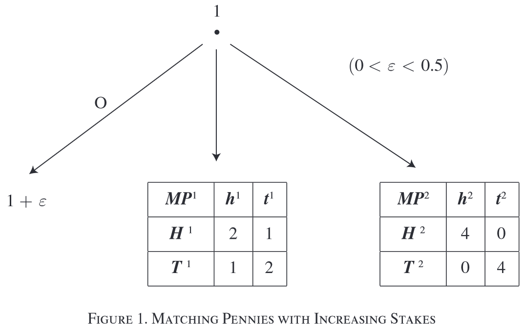
Player 1 chooses between an outside option and two Matching Pennies Games and

• Subgame has higher maxmin stakes than (maxmin value )
  • Calculate the maxmin value: in the distribution that minimize the expected payoff is , in which the highest payoff (maxmin value) is 2. Similarly, maxmin value in is 1.5.
• only one Bayesian SCE: Player 1 always choose due to a higher maxmin value and one half of players play
• sub prob of P1:  assign probability to the choice as  , and
  • subjective value: in and in
  • However, the value of is , which is lower than other two Games

What Subgames are reachable?

• For an ambiguity neutral agent, neither nor can happen in a Bayesian SCE
  • in a repeated game. even if they are inor, they can learn and turn to
• Ambiguity aversion makes or reachable through status quo bias
  • For agents already in with moderate ambiguity aversion, the aversion to unknown payoff in case makes its payoff penalized, so people still stay in
  • High ambiguity aversion makes the option also possible since people in do not want to suffer from ambiguity in both games. For an extreme case, the agent see obj payoff in as the lowest payoff 1 and as the lowest payoff 0, which are less than

Recurrent Games and Self-Confirming Equilibrium ​

Games with Feedback ​

a game form with feedback has the form：

• is the set of player roles
• is the finite set of strategies of , and let and denote the set of all strategy files and player’s opponents’ strategies
• is a set of messages that playermay receive at the end of the game
• Feedback function: . If the game is dynamic, a player’s feedback is a function of the terminal node reached under strategy profile . In this case, where is the extensive-form feedback function for player .

Example 1: Three cases about the forms of Feedback

1. each player observes the terminal node (reached under the realized strategy profile). That is, is the identity on
2. each player observes everybody’s material consequences at the terminal node, that is, is the consequence function
3. each player observes his own material consequences at the terminal node, that is, is the projection of

The player infer that the strategy profile played by his opponents must belong to the set

Rewrite:

Example 2: in former game, player 1 observes only his monetary payoff

the ex post information partition:

Note. A game form with feedback satisfies own-strategy independence of feedback if the ex post information partition $ F*{s_i}$ is independent of for every . This property is very strong and is violated in many interesting cases.

Players' Preferences ​

For , we have:

Call game with feedback the tuple

Ambiguity Aversion (KMM smooth ambiguity criterion)

ambiguity attitudes in population i are represented by a strictly increasing and continuous function , where

KMM smooth ambiguity criterion is

• player is uncertain about the true distribution of strategies in the population of potential opponents
• measure of ambiguity aversion:

von-Neumann Utility in KMM

standard Bayesian SEU in KMM

robust criterion Gilboa and Schmeidler